Exploring Financial Predictions with Python: A Deep Dive into Autodesk's Stock

In the realm of financial analysis and prediction, Python emerges as a powerful tool, offering clarity and precision in navigating the complexities of stock market data. This post delves into a comprehensive Python script designed to analyze and predict Autodesk’s stock prices, leveraging a variety of data science and machine learning techniques.

The Problem at Hand

Why Autodesk, and why now? As a leader in design software, Autodesk’s stock (ADSK) is a reflection of its innovative capabilities and market position. However, like all stocks, it is subject to the ebb and flow of market forces. Investors seeking to optimize their portfolios need to look ahead, beyond current trends, to anticipate the potential growth or decline in stock value. This is where predictive modeling comes into play, offering a window into the future based on historical data patterns.

The Importance of Prediction

The task at hand is two-fold: to demonstrate the potential of Python in extracting actionable insights from historical price data and to provide a 10-day forecast that could guide investment strategies. But the implications extend beyond Autodesk. The models and methods employed here are transferable to other stocks, enabling analysts to apply similar techniques to a broad spectrum of investment opportunities. Whether for individual stock selection, portfolio management, or risk assessment, the ability to project future price movements is invaluable.

Broader Applications

The linear regression model we’ll explore is not confined to the world of finance. Its applications span across various domains where forecasting is crucial—be it weather prediction, supply chain management, or even sports analytics. Anywhere that historical data can be harnessed to predict future events, linear regression can be a key player in the analytical toolkit.

Data Acquisition and Preparation

The journey begins with the yfinance library, a Python package that allows users to download historical stock price data. By specifying a ticker symbol, such as Autodesk’s “ADSK”, and a date range, we can retrieve a dataset comprising open, high, low, close, and volume information. The initial step involves augmenting this dataset with daily returns and the next day’s price, enriching the data for more insightful analysis.

Visual Analytics

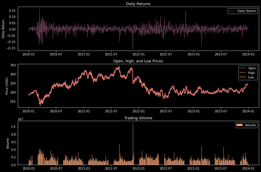
Visualization plays a crucial role in financial analysis. The script employs matplotlib to craft three distinct types of charts: daily returns, stock price movements (open, high, low), and trading volume. These visualizations offer a multifaceted view of Autodesk’s stock performance, highlighting trends and patterns that might not be immediately evident from raw data alone.

def plot_stock_data(data, colors):
    plt.style.use('dark_background')
    fig, axs = plt.subplots(3, 1, figsize=(12, 8))
    
    # Configuration
    plot_configs = [
      {'data_col': 'Daily_Return', 'ax': axs[0], 'label': 'Daily Return', 'title': 'Daily Returns', 'ylabel': 'Daily Return', 'color': colors['daily_return']},
      {'data_col': 'Open', 'ax': axs[1], 'label': 'Open', 'title': 'Open, High, and Low Prices', 'ylabel': 'Price (USD)', 'color': colors['open']},
      {'data_col': 'High', 'ax': axs[1], 'label': 'High', 'color': colors['high']},
      {'data_col': 'Low', 'ax': axs[1], 'label': 'Low', 'color': colors['low']},
      {'data_col': 'Volume', 'ax': axs[2], 'label': 'Volume', 'title': 'Trading Volume', 'ylabel': 'Volume', 'color': colors['volume'], 'bar': True},
    ]


    for config in plot_configs:
        if 'bar' in config:
            config['ax'].bar(data.index, data[config['data_col']], label=config['label'], color=config['color'])
        else:
            config['ax'].plot(data.index, data[config['data_col']], label=config['label'], color=config['color'])
        
        if 'title' in config:
            config['ax'].set_title(config['title'])
        if 'ylabel' in config:
            config['ax'].set_ylabel(config['ylabel'])
        config['ax'].legend()
    
    plt.tight_layout()

Predictive Modeling with Linear Regression

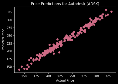
At the core of this analysis is the linear regression model, a fundamental tool in predictive analytics. By training this model on Autodesk’s historical stock data, we can uncover relationships between various features (such as opening price, highest price of the day, and daily returns) and the next day’s closing price. The model’s predictions, alongside metrics like mean squared error (MSE) and R-squared (R²), provide insights into its accuracy and efficacy.

def linear_regression_model(data, colors):
    X = data[['Open', 'High', 'Low', 'Volume', 'Daily_Return']]
    y = data['Next_Day_Price']
    X_train, X_test, y_train, y_test = train_test_split(X, y, test_size=0.2, random_state=42)

    model = LinearRegression()
    model.fit(X_train, y_train)
    y_pred = model.predict(X_test)
    
    mse = mean_squared_error(y_test, y_pred)
    r2 = r2_score(y_test, y_pred)
    print(f'Mean Squared Error (MSE): {mse}')
    print(f'R-squared (R^2): {r2}')

    # Visualizar los resultados de la regresión
    plot_regression_results(y_test, y_pred, colors)

    return model

Future Price Predictions

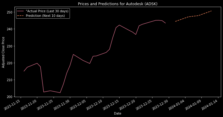
The script takes a bold step forward by forecasting Autodesk’s stock prices for the next 10 business days. It cleverly extrapolates future prices based on the average percentage change of the last five days, offering a glimpse into potential future trends. This predictive feature is not only a testament to the power of Python and linear regression in financial analysis but also a valuable asset for investors and analysts looking to make informed decisions.

Visualization of Predictions

The culmination of this analysis is the visualization of both historical price data and future price predictions. This final chart juxtaposes the actual stock prices with the predicted values, providing a clear and compelling representation of the model’s predictive capabilities and the stock’s potential future movements.

def predict_future_prices(model, data, colors):
    last_day = data.index[-1]
    new_dates = [last_day + BDay(i) for i in range(1, 11)]

    # Calcular el cambio porcentual promedio de los últimos 5 días
    mean_percentage_change = data[['Open', 'High', 'Low', 'Volume', 'Daily_Return']].pct_change().rolling(window=5).mean().iloc[-1]

    # Inicializar un DataFrame para las características futuras
    future_features = pd.DataFrame(index=new_dates, columns=['Open', 'High', 'Low', 'Volume', 'Daily_Return'])
    
    # Aplicar la extrapolación basada en el cambio porcentual promedio
    for i, date in enumerate(future_features.index):
        if i == 0:
            future_features.loc[date] = data[['Open', 'High', 'Low', 'Volume', 'Daily_Return']].iloc[-1]
        else:
            future_features.loc[date] = future_features.iloc[i-1] * (1 + mean_percentage_change)

    future_features = future_features.astype(float)

    # Realizar predicciones con el modelo
    future_predicted_prices = model.predict(future_features)

    # Crear un DataFrame para las fechas y precios pronosticados
    predictions_df = pd.DataFrame({'Date': new_dates, 'Predicted_Price': future_predicted_prices})

    print(predictions_df)

Conclusion

In conclusion, this Python script embodies the intersection of data science and financial analysis, offering a robust framework for stock price prediction. Through meticulous data preparation, insightful visualization, and sophisticated predictive modeling, it paves the way for data-driven investment strategies and financial insights.